
13.6. 最小生成树
13.6.1. 最小生成树
最小生成树 (MCST)问题以连通的无向图 \(\mathbf{G}\) 作为输入,其中每条边都有距离或权值度量。 MCST 是包含 \(\mathbf{G}\) 的顶点以及 \(\mathbf{G}\) 的边子集的图,该子集 (1) 具有通过求和子集中所有边值来衡量的最小总成本,以及 (2) 保持顶点连通。此问题的解决方案有用的应用包括焊接连接电路板上一组端子所需的最短线束,以及通过电话线连接一组城市,以所需最少的电缆量。
MCST 不包含环。如果建议的 MCST 确实有环,可以通过删除环中的任何一条边来获得更便宜的 MCST。因此,MCST 是具有 \(|\mathbf{V}| - 1\) 条边的自由树。 "最小生成树"这个名字来源于所需的边集形成一棵树、它跨越顶点(即连接它们),并且具有最小成本。图 13.6.1 显示了一个示例图的 MCST。
13.6.1.1. Prim 算法
我们两个 MCST 算法中的第一个通常被称为 Prim 算法。 Prim 算法非常简单。从图中的任何顶点 \(N\) 开始,最初将 MCST 设为 \(N\)。选择连接 \(N\) 的最小成本边。这条边将 \(N\) 连接到另一个顶点;称它为 \(M\)。将顶点 \(M\) 和边 \((N, M)\) 添加到 MCST。接下来,选择从 \(N\) 或 \(M\) 到图中任何其他顶点的最小成本边。将此边及其到达的新顶点添加到 MCST。此过程继续,每一步通过选择从当前在 MCST 中的顶点到当前不在 MCST 中的顶点的最小成本边来扩展 MCST。
Prim 算法与 Dijkstra 的单源最短路径算法非常相似。主要区别在于我们寻找的不是距离起始顶点最近的下一个顶点,而是距离当前在 MCST 中任何顶点最近的下一个顶点。因此我们替换以下行:
if (D[w] > (D[v] + G.weight(v, w)))
  D[w] = D[v] + G.weight(v, w);
在 Dijkstra 算法中,替换为以下行:
if (D[w] > G.weight(v, w))
  D[w] = G.weight(v, w);
在 Prim 算法中。
以下代码展示了 Prim 算法的实现,它在距离矩阵中搜索下一个最近的顶点。
// Compute shortest distances to the MCST, store them in D.
// V[i] will hold the index for the vertex that is i's parent in the MCST
void Prim(Graph G, int s, int[] D, int[] V) {
  for (int i=0; i<G.nodeCount(); i++) {    // Initialize
    D[i] = INFINITY;
  }
  D[s] = 0;
  for (int i=0; i<G.nodeCount(); i++) {  // Process the vertices
    int v = minVertex(G, D);     // Find next-closest vertex
    G.setValue(v, VISITED);
    if (D[v] == INFINITY) { return; } // Unreachable
    if (v != s) { AddEdgetoMST(V[v], v); }
    int[] nList = G.neighbors(v);
    for (int j=0; j<nList.length; j++) {
      int w = nList[j];
      if (D[w] > G.weight(v, w)) {
        D[w] = G.weight(v, w);
        V[w] = v;
      }
    }
  }
}
// Compute shortest distances to the MCST, store them in D.
// V[i] will hold the index for the vertex that is i's parent in the MCST
void Prim(Graph G, int s, int[] D, int[] V) {
  for (int i=0; i<G.nodeCount(); i++) {    // Initialize
    D[i] = INFINITY;
  }
  D[s] = 0;
  for (int i=0; i<G.nodeCount(); i++) {  // Process the vertices
    int v = minVertex(G, D);     // Find next-closest vertex
    G.setValue(v, VISITED);
    if (D[v] == INFINITY) { return; } // Unreachable
    if (v != s) { AddEdgetoMST(V[v], v); }
    int[] nList = G.neighbors(v);
    for (int j=0; j<nList.length; j++) {
      int w = nList[j];
      if (D[w] > G.weight(v, w)) {
        D[w] = G.weight(v, w);
        V[w] = v;
      }
    }
  }
}
对于每个顶点 \(I\),当 \(I\) 被 Prim 算法处理时,一条指向 \(I\) 的边被添加到我们正在构建的 MCST 中。数组 V[I] 存储之前访问过的距离顶点 I 最近的顶点。此信息让我们知道当处理顶点 \(I\) 时哪条边进入 MCST。上面的实现还包含对 AddEdgetoMST 的调用,以指示哪些边实际被添加到 MCST。


13.6.1.2. Prim 算法的另一种实现
或者,我们可以使用 优先队列 来实现 Prim 算法以找到下一个最近的顶点,如下所示。与 Dijkstra 算法的优先队列版本一样, 堆 存储 DijkElem 对象。
// Prims MCST algorithm: priority queue version
void PrimPQ(Graph G, int s, int[] D, int[] V) {
  int v;                                 // The current vertex
  KVPair[] E = new KVPair[G.edgeCount()];        // Heap for edges
  E[0] = new KVPair(0, s);               // Initial vertex
  MinHeap H = new MinHeap(E, 1, G.edgeCount());
  for (int i=0; i<G.nodeCount(); i++) {            // Initialize distance
    D[i] = INFINITY;
  }
  D[s] = 0;
  for (int i=0; i<G.nodeCount(); i++) {          // For each vertex
    KVPair temp = H.removemin();
    if (temp == null) { return; }      // Unreachable nodes exist
    v = (Integer)temp.value();
      while (G.getValue(v) == VISITED) {
        KVPair temp = H.removemin();
        if (temp == null) { return; }      // Unreachable nodes exist
        v = (Integer)temp.value();
      }
    G.setValue(v, VISITED);
    if (D[v] == INFINITY) { return; }  // Unreachable
    if (v != s) { AddEdgetoMST(V[v], v); } // Add edge to MST
    int[] nList = G.neighbors(v);
    for (int j=0; j<nList.length; j++) {
      int w = nList[j];
      if (D[w] > G.weight(v, w)) { // Update D
        D[w] = G.weight(v, w);
        V[w] = v;                  // Where it came from
        H.insert(D[w], w);
      }
    }
  }
}
// Prims MCST algorithm: priority queue version
void PrimPQ(Graph G, int s, int[] D, int[] V) {
  int v;                                 // The current vertex
  KVPair[] E = new KVPair[G.edgeCount()];        // Heap for edges
  E[0] = new KVPair(0, s);               // Initial vertex
  MinHeap H = new MinHeap(E, 1, G.edgeCount());
  for (int i=0; i<G.nodeCount(); i++) {            // Initialize distance
    D[i] = INFINITY;
  }
  D[s] = 0;
  for (int i=0; i<G.nodeCount(); i++) {          // For each vertex
    KVPair temp = H.removemin();
    if (temp == null) { return; }      // Unreachable nodes exist
    v = (Integer)temp.value();
      while (G.getValue(v) == VISITED) {
        KVPair temp = H.removemin();
        if (temp == null) { return; }      // Unreachable nodes exist
        v = (Integer)temp.value();
      }
    G.setValue(v, VISITED);
    if (D[v] == INFINITY) { return; }  // Unreachable
    if (v != s) { AddEdgetoMST(V[v], v); } // Add edge to MST
    int[] nList = G.neighbors(v);
    for (int j=0; j<nList.length; j++) {
      int w = nList[j];
      if (D[w] > G.weight(v, w)) { // Update D
        D[w] = G.weight(v, w);
        V[w] = v;                  // Where it came from
        H.insert(D[w], w);
      }
    }
  }
}
Prim 算法是贪心算法的一个例子。在 for 循环的每一步中,我们选择连接某个已标记顶点与某个未标记顶点的成本最低的边。该算法不会进一步检查最小生成树是否真的应该包含这条成本最低的边。这就引出了一个重要问题:Prim 算法是否正确?显然,它会生成一棵生成树(因为 for 循环的每次迭代都会向生成树中添加一条边和一个未标记顶点,直到所有顶点都被加入),但这棵树的成本是最小的吗?
定理: Prim 算法产生最小生成树。
证明: 我们将使用反证法。设 \(\mathbf{G} = (\mathbf{V}, \mathbf{E})\) 是一个图,对于该图 Prim 算法 没有 生成 MCST。根据 Prim 算法将顶点添加到 MCST 的顺序定义顶点的排序: \(v_0, v_1, ..., v_{n-1}\)。设边 \(e_i\) 连接 \((v_x, v_i)\),其中某个 \(x < i\) 且 \(i \leq 1\)。设 \(e_j\) 是 Prim 算法添加的第一个(编号最小的)边,使得到目前为止选择的边集 无法 扩展以形成 \(\mathbf{G}\) 的 MCST。换句话说,\(e_j\) 是 Prim 算法"出错"的第一条边。设 \(\mathbf{T}\) 是"真正的" MCST。称 \(v_p (p<j)\) 为由边 \(e_j\) 连接的顶点,即 \(e_j = (v_p, v_j)\)。
因为 \(\mathbf{T}\) 是一棵树,在 \(\mathbf{T}\) 中存在某条连接 \(v_p\) 和 \(v_j\) 的路径。这条路径中必须有某条边 \(e'\) 连接顶点 \(v_u\) 和 \(v_w\),其中 \(u < j\) 且 \(w \geq j\)。因为 \(e_j\) 不是 \(\mathbf{T}\) 的一部分,将边 \(e_j\) 添加到 \(\mathbf{T}\) 会形成一个环。边 \(e'\) 的成本必须低于边 \(e_j\),因为 Prim 算法没有生成 MCST。此情况如图 13.6.2 所示。然而,Prim 算法会选择可用的最小成本边。它会选择 \(e'\),而不是 \(e_j\)。因此,Prim 算法选择了错误的边是矛盾的,所以 Prim 算法一定是正确的。证毕
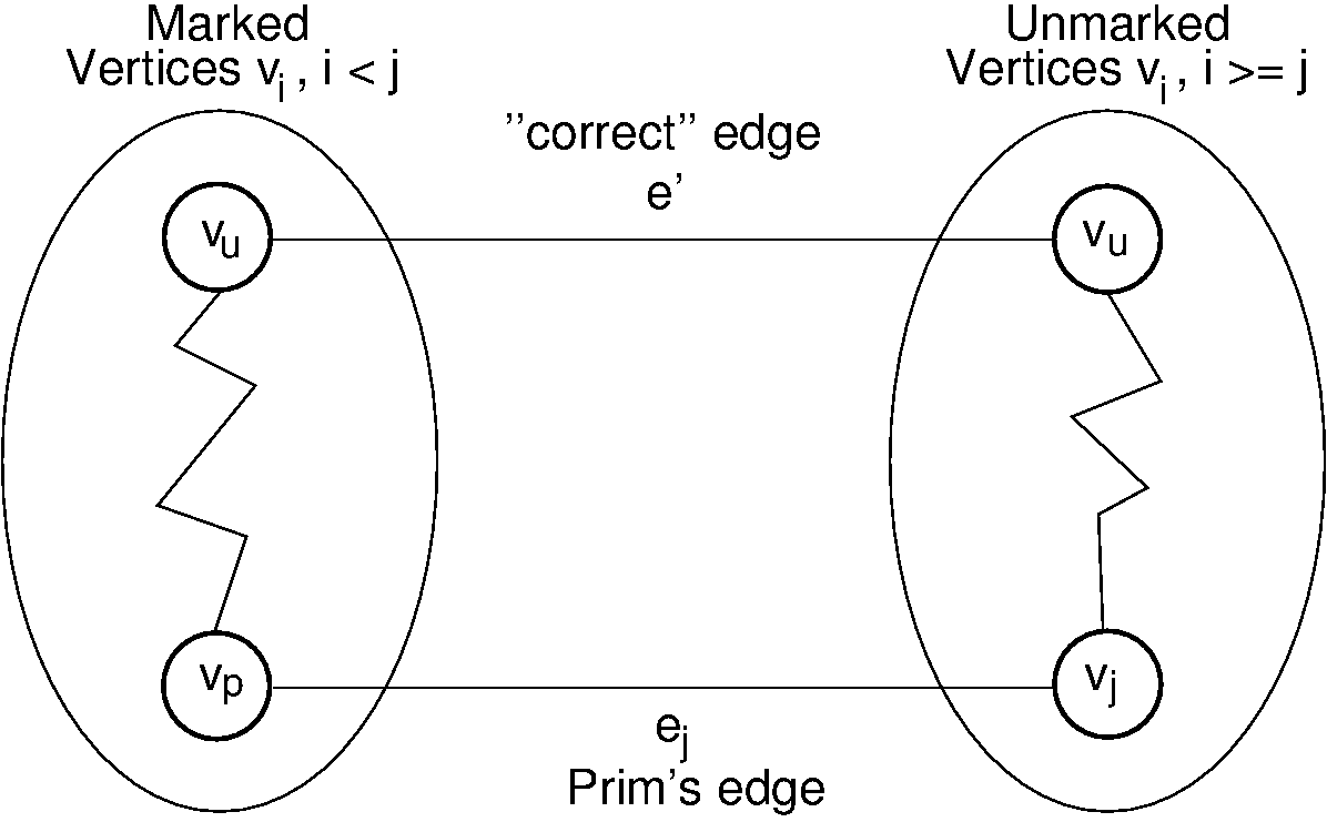
Figure 13.6.1: Prim 的 MCST 算法证明。左边的椭圆包含 Prim 的 MCST 和"真正的" MCST \(\mathbf{T}\) 一致的部分。右边的椭圆包含图的其余部分。图的两部分通过(至少)边 \(e_j\) (由 Prim 算法选择在 MCST 中)和 \(e'\) (要放在 MCST 中的"正确"边)连接。注意从 \(v_w\) 到 \(v_j\) 的路径不能包含任何已标记顶点 \(v_i, i \leq j\),因为这样做会形成一个环。